
Testing the RSI Indicator with Bayesian Estimation
I previously tested the RSI indicator against the Dow Jones Industrial Average using ordinary high school statistics. In this post I'll be pulling out my big guns: Bayesian estimation.
This is an approach that respects the statistical nature of the variables in question. Every value is a slice of a probability distribution. It works on those distributions of possible values, rather than the individual values themselves.
Tested Allegation
The probability distribution of the next-day returns following an overbought day is different from a non-overbought day.
Parameters
14 day period (industry standard)
RSI value of 70 is overbought
Time Period
One trading day. The signal value at end of day is assumed to affect the end of day return for the following trading day.
Data and Priors
Data used is the Dow Jones Industrial Average daily close from 1928-09-30 to 2020-07-30.
Bayesian Estimation Priors
Bayesian analysis begins with "priors". These are initial values for the probability distributions. These priors will be adjusted by the real data to obtain the posteriors which our best guesses for the true distributions given the data.
The following day returns for both the overbought and non-overbought series follow the StudentT distribution.
The mean values of these distributions follow a normal distribution. These are initialized with the mean and standard deviation for the overall return series
The standard deviation of the return series follow a uniform distribution between 0.001% and 100%. This is called a "naive" prior, because it's not much of an assumption, it's more of a shrug 🤷♀️
Method
Bayesian estimation using the pymc3 library. It uses a No-U-Turn sampling algorithm (NUTS) which is a gradient based Markov chain Monte Carlo (MCMC) sampling algorithm that is used to sample from a probability distribution.
That's a lot of fancy words. The specifics of the NUTS algorithm itself are not too important; it's used because it's fast. Here's an article about MCMC that might help you wrap your head around what's going on here.
Ultimately we use this approach to build a posterior probability distribution for the return series following overbought and non-overbought days. We then plot the difference between those two probability distributions and evaluate if the results are significant.
Results
A fun part of using Bayesian estimation for analysis is the results are readily presentable graphically. In the following graphics "trigger" means overbought and non-trigger means not overbought.
Charts
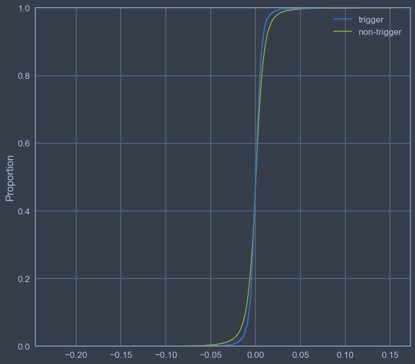
This first chart shows the difference between the two return distributions. The proportion axis tells you how much of the data (next day returns) fall below the x-axis value.
The non-trigger returns demonstrate a wider range of extreme values - but that's to be expected. In this data set, we have 2,360 overbought conditions and 20,686 non-trigger conditions. Other than that, these distributions look the same.
The next chart shows the difference in the mean value and the standard deviation for the return series. These are both modeled as probability distributions, and so their difference is itself a probability distribution. The black bar at the bottom is the 94% high density interval (HDI), which is analogous to a confidence interval except much more directly intuitive.

The sensitivity index plot is an indication of how seriously we should take any detected difference between the distributions. There's no perfect rule on how to use it, but its similar to a Z-score in how its magnitude is interpreted.

Conclusions
In this result, we see that there is no significant difference between the means of the two return series. The average value is a very confident 0. The average return for the day following an overbought day is not different from the average return for a non-overbought day.
Based on the HDI, there is a significant difference in the standard deviation between these two distributions, but the detected difference is a very small -0.2%.
The sensitivity index does not provide strong support for this difference in the standard deviation being significant. A Z-score of 0.039 translates to a confidence interval of approximately 3%.
The difference in standard deviations is attributable to the sample size of the two sets. We had only 2,360 overbought days and 20,686 non-overbought days. More days in the market implies exposure to more volatility.
Just like in our much simpler analysis, we can only conclude that an RSI overbought condition using a 14-day period had no bearing whatsoever on the following trading day's return for these data and parameters.
RSI is noise, not signal. (for this set of parameters and data)